Plotting Fresnel Equation

Introduction: Simple Equation Derivation

We start with Fresnel Equations

where

$$ \alpha\equiv \frac{\cos\theta_T}{\cos\theta_I}, \tag{2} $$

and

$$ \beta \equiv \frac{\mu_1 v_1}{\mu_2 v_2} = \frac{\mu_1 n_2}{\mu_2 n_1}. \tag{3} $$

If we assume the special case where $\mu_1 \cong \mu_2 \cong \mu_0$ then

$$ \beta \cong \frac{n_2}{n_1}. \tag{4} $$

Based on Snell’s law we know that

$$ \sin\theta_T = \frac{n_1}{n_2} \sin\theta_I. \tag{5} $$

Using identity $\cos^2\theta_T+\sin^2\theta_T = 1$ then the previous $ \alpha $ equation (2) becomes

$$ \alpha = \frac{\sqrt{1-\sin^2\theta_T}}{\cos\theta_I} = \frac{\sqrt{1-\left[(n_1/n_2)\sin\theta_I\right]^2}}{\cos\theta_I}. $$

For reflectance and transmittance

Source Code

https://github.com/firman-qs/fresnel-equation-plot-python.

"""
FRESNEL EQUATION PLOT.

Today we will plot FRESNEL EQUATION.
Required libraries: NumPy and Matplotlib.
"""

# Import Library
import numpy as np
import matplotlib.pyplot as plt
import matplotlib

"""
For mathematical beauty, if you have, you can use latex fonts.
"""
rc_fonts = {
    "text.usetex": True,
    "font.size": 14,
    "mathtext.default": "regular",
    "axes.titlesize": 15,
    "axes.labelsize": 15,
    "legend.fontsize": 14,
    "xtick.labelsize": 14,
    "ytick.labelsize": 14,
    "figure.titlesize": 15,
    "text.latex.preamble": r"\usepackage{amsmath,amssymb,bm,physics,lmodern}",
    "font.family": "serif",
    "font.serif": "computer modern roman",
}
matplotlib.rcParams.update(rc_fonts)

"""
First we determine the refractive index of the medium,
for example from air (1.0) to glass (1.5).
"""
n_1 = 1.0  # refractive index of air
n_2 = 1.5  # refractive index of glass


def alphaAndBeta(theta_i):
    '''
    Function that returns alpha (as a function of the angle of incidence) and 
    beta (you can see equations 9.106 and 9.108 in Griffiths's book Introduction
    to Electrodynamics)
    '''
    alpha = (np.sqrt(1-((n_1/n_2)*np.sin(theta_i))**2))/(np.cos(theta_i))
    beta = n_2/n_1
    return alpha, beta


def reflectionAndTransmissionCoefficient(theta_i):
    '''
    Function that returns the reflection coefficient and transmission coefficient
    (you can read the Fresnel equation (Equation 9.109) in Griffiths's book:
    Introduction to Electrodynamics).
    '''
    alpha = alphaAndBeta(theta_i)[0]
    beta = alphaAndBeta(theta_i)[1]
    # (Equation 9.109 Griffith Introduction to Electrodynamics).
    reflection_coefficient = (alpha-beta)/(alpha+beta)
    transmission_coefficient = 2/(alpha+beta)
    return reflection_coefficient, transmission_coefficient


def reflectanceAndTransmittance(theta_i):
    """ Reflectance and Transmittance Function.

    A function that returns the transmittance reflectance (Equation 9.115 & 9.116
    in Griffiths's book Introduction to Electrodynamics).
    """
    alpha = alphaAndBeta(theta_i)[0]
    beta = alphaAndBeta(theta_i)[1]
    # (Equation 9.115 & 9.116 Griffith Introduction to Electrodynamics).
    reflectance = ((alpha-beta)/(alpha+beta))**2
    transmittance = alpha*beta*((2/(alpha+beta))**2)
    return reflectance, transmittance


# Creates an array of theta_i axis values
theta_range = np.radians(np.linspace(0, 100, 100))

# Create an array of transmission & reflection coefficient values ​​for each
# theta_i in theta_range
reflection_coefficient = np.array(
    [reflectionAndTransmissionCoefficient(theta)[0] for theta in theta_range])
transmission_coefficient = np.array(
    [reflectionAndTransmissionCoefficient(theta)[1] for theta in theta_range])

# Create an array of transmittance & reflectance values ​​for each theta_i
# in theta_range
reflectance = np.array([reflectanceAndTransmittance(theta)[0]
                        for theta in theta_range])
transmittance = np.array([reflectanceAndTransmittance(theta)[1]
                          for theta in theta_range])

# Brewster's angle
theta_brewster = np.degrees(np.arctan(n_2/n_1))

# Tick for x-axis and y-axis
ticks_x = np.setdiff1d(np.append(np.arange(0, 90, 10),
                       np.round([theta_brewster], 3)), [50, 60])
ticks_y = np.arange(-0.4, 1, 0.2)

'''
Plot of Reflection and Transmission Coefficients
'''
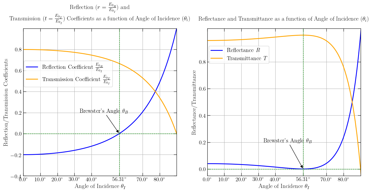
figure, (graph_1, graph_2) = plt.subplots(1, 2, figsize=(12, 6))
graph_1.plot(np.degrees(theta_range), reflection_coefficient,
             label=r'Reflection Coefficient $\frac{E_{0_R}}{E_{0_I}}$', linewidth=2, color='blue')
graph_1.plot(np.degrees(theta_range), transmission_coefficient,
             label=r'Transmission Coefficient $\frac{E_{0_T}}{E_{0_I}}$', linewidth=2, color='orange')
graph_1.set_xlabel(r'Angle of Incidence $\theta_I$')
graph_1.set_ylabel('Reflection/Transmission Coefficients')
graph_1.set_yticks(ticks=ticks_y)
graph_1.set_title(r'''Reflection ($r=\frac{E_{0_R}}{E_{0_I}}$) and
Transmission ($t=\frac{E_{0_T}}{E_{0_I}}$) Coefficients as a function of Angle of Incidence ($\theta_i$)''', pad=20)
graph_1.axis([0, 90, -0.4, 1.0])
graph_1.tick_params(top=True, right=True, direction="in", length=7, width=0.9)
graph_1.legend(loc="upper right", bbox_to_anchor=(0.6, 0.8))


'''
Transmittance & Reflectance Plot
'''
graph_2.plot(np.degrees(theta_range), reflectance,
             label=r'Reflectance $R$', linewidth=2, color='blue')
graph_2.plot(np.degrees(theta_range), transmittance,
             label=r'Transmittance $T$', linewidth=2, color='orange')
graph_2.set_xlabel(r'Angle of Incidence $\theta_I$')
graph_2.set_ylabel('Reflectance/Transmittance')
graph_2.set_yticks(ticks=ticks_y)
graph_2.set_title(
    r'Reflectance and Transmittance as a function of Angle of Incidence ($\theta_i$)', pad=20)
graph_2.axis([0, 90, -0.05, 1.05])
graph_2.tick_params(top=True, right=True, direction="in", length=7, width=0.9)
graph_2.legend(loc="upper right", bbox_to_anchor=(0.42, 0.9))

# General Properties of Graph 1 & 2
for i in range(2):
    locals()[f"graph_{i+1}"].grid()
    locals()[f"graph_{i+1}"].annotate(r"Brewster's Angle $\theta_B$",
                                      xy=(np.degrees(np.arctan(n_2/n_1)), 0.0), xytext=(33, 0.2),
                                      arrowprops={"arrowstyle": "-|>", "color": "black"})
    locals()[f"graph_{i+1}"].set_xticks(ticks_x,
                                        [r"${angle}^\circ$".format(angle=angle) for angle in ticks_x])
    locals()[f"graph_{i+1}"].axhline(0.0,
                                     linewidth=1, color='green', linestyle='--')
    locals()[f"graph_{i+1}"].axvline(np.degrees(np.arctan(n_2/n_1)),
                                     linewidth=1, color='green', linestyle='--')

# Axis thickness
for axis in ['top', 'bottom', 'left', 'right']:
    graph_1.spines[axis].set_linewidth(0.9)
    graph_2.spines[axis].set_linewidth(0.9)

# Subplots settings
plt.subplots_adjust(left=0.1,
                    bottom=0.1,
                    right=0.95,
                    top=0.84,
                    wspace=0.2,
                    hspace=0.1)

plt.show()
# Save plot to png file.
figure.savefig("fresnel_equation_plot_python.png", bbox_inches='tight')

Final Result

Video on Plotting Fresnel Equations